Intro to Big O Notation
On This Page View Sections
Note: A more detailed dive on the topic can be found in my old site’s blog
1k2s.netlify.app. This page goes over the same topic but in a more succinct matter.
Big Notation is a mathematical notation that describes the behavior of a value (most commonly denoted as as it reaches infinity. Although well defined as such in math, applied in programming it comes in 2 forms Time Complexity and Space Complexity.
Dictionary
- Time Complexity: Used to determine how much time it takes for the CPU to run the code.
- Space Complexity: Memory resources needed to complete the algorithm.
- Compile Time: This is not measured with Big O, instead we care about runtime, and even though some algorithms can be optimized from to (like Gauss Sum for example, this blog doesn’t go over these kinds of optimizations.
- Runtime: When the program is actually executed. This is what LeetCode and other platforms alike measure.
Analysis
Below are the most common algorithm complexities listed, in general it’s important to know that when assessing an algorithm’s complexity, we omit all constants and instead focus on how the algorithm works as the input increases in size.
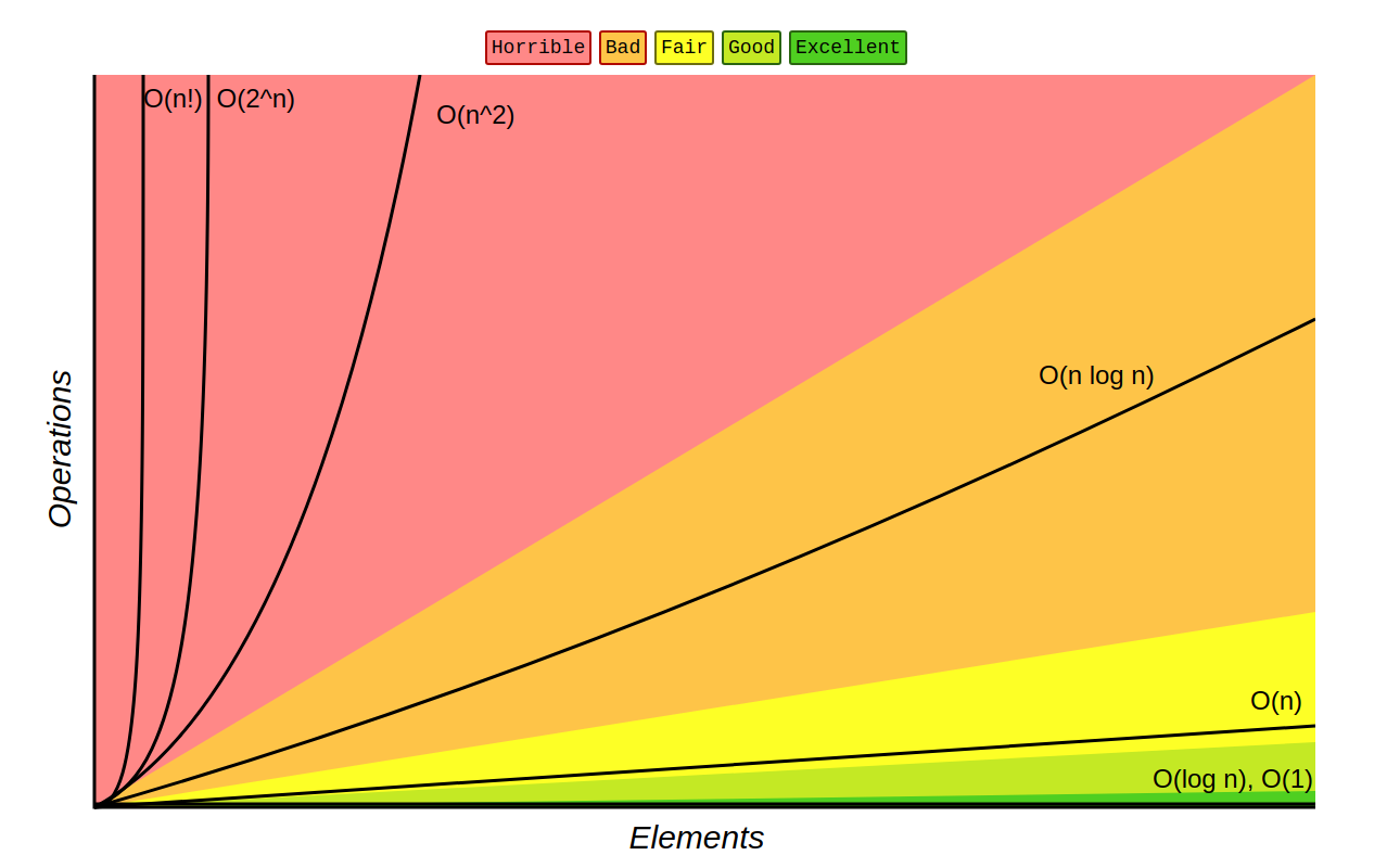
- Constant Complexity
Seen in:
- Pushing an item to the back of a Vector.
- Looking up an item in a Hash Map/Set.
- Getting the first element of a Linked List.
- Logarithmic Complexity
The concept is as follows: if you divide the amount of steps required by (most of the time ) on every iteration, then your algorithm’s time complexity is .
Primary use is Binary Search. It is the gold standard for searching sorted data sets.
- Linear Complexity
Described as doing at least one full iteration on your data.
Note: A common trick question is removing the first item of a Vector is , unlike removing the last one which is . This is due to how Vectors are structured in memory and how every subsequent item needs to be moved forward whenever you remove at the first place.
- Linearithmic Complexity
Usually where efficient sorting algorithms fall: Quicksort, Heapsort, and Merge sort, all in regards to time complexity.
- Quadratic Complexity
Commonly seen in nested loops or matrix traversals (arr[i][j]). Bubble Sort
also falls here.
Note: Often solutions are referred to as Brute Force. A common approach to optimizing such problems is called Dynamic Programming.
Complexity Table
In for easy reference you could refer to it:
| Complexity | Example | Intuition |
|---|---|---|
| array access | constant | |
| binary search | halves each step | |
| linear scan | proportional | |
| nested loops | pair comparisons |
Code Implementation Examples
import math

# O(1) - Constant Time
# No matter how large the input 'arr' is, this takes one step.
def constant_example(arr):
    return arr[0] if arr else None

# O(log n) - Logarithmic Time
# Binary Search: Cutting the search area in half each iteration.
def logarithmic_example(arr, target):
    low, high = 0, len(arr) - 1
    while low <= high:
        mid = (low + high) // 2
        if arr[mid] == target:
            return mid
        elif arr[mid] < target:
            low = mid + 1
        else:
            high = mid - 1
    return -1

# O(n) - Linear Time
# A single loop that visits every element once.
def linear_example(arr):
    for item in arr:
        print(item)

# O(n log n) - Linearithmic Time
# Typical for efficient sorts like Merge Sort.
def linearithmic_example(arr):
    if len(arr) <= 1:
        return arr
    mid = len(arr) // 2
    left = linearithmic_example(arr[:mid])
    right = linearithmic_example(arr[mid:])
    return sorted(left + right) # Simplified merge step

# O(n^2) - Quadratic Time
# Nested loops where we compare every element to every other element.
def quadratic_example(arr):
    n = len(arr)
    for i in range(n):
        for j in range(n):
            print(f"Comparing {arr[i]} and {arr[j]}")

# O(sqrt(n)) - Sublinear Time
# Trial division for primality testing.
def sqrt_n_example(n):
    if n < 2: return False
    for i in range(2, int(math.sqrt(n)) + 1):
        if n % i == 0:
            return False
    return True
Optimizing for Memory vs. Space
Below is a video with a very comprehensive showcase of all three approaces: Trial Division, Sieve of Eratosthenes, and Dijkstra’s Approach.
1. Trial Division
The most memory-efficient but slowest method. It relies on the fact that divisors are mirrored around the square root of .
- Time: <<= on theory, good, in reality the slowness is due to Integer Factorization.
- Space:
2. Sieve of Eratosthenes
The quickest for bulk evaluation.
- Time:
- Space: (requires a boolean array up to )
3. Dijkstra’s Approach
A balanced approach using a “pool” of tuples to track multiples, avoiding the massive memory hit of the Sieve while staying faster than Trial Division.
- Time: <<= whilst sharing the same time complexity as Sieve of Eratosthenes, it usually performs slower due to Cache Locality.
- Space: (requires a boolean array up to )
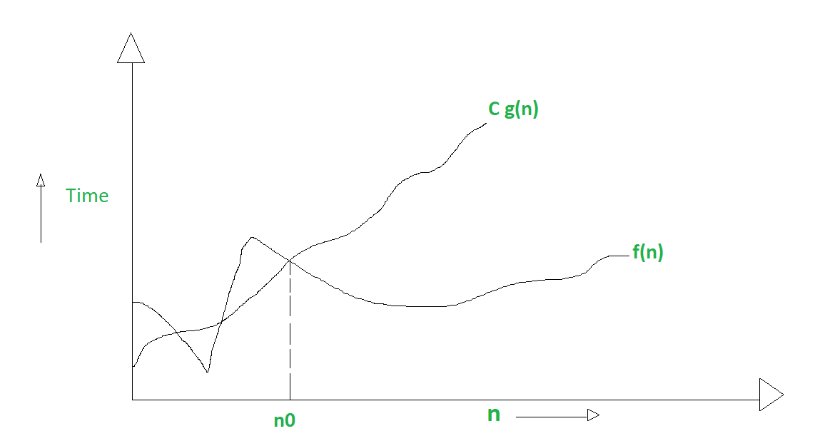
Not only Big
Big describes the worst-case scenario. Mathematically:
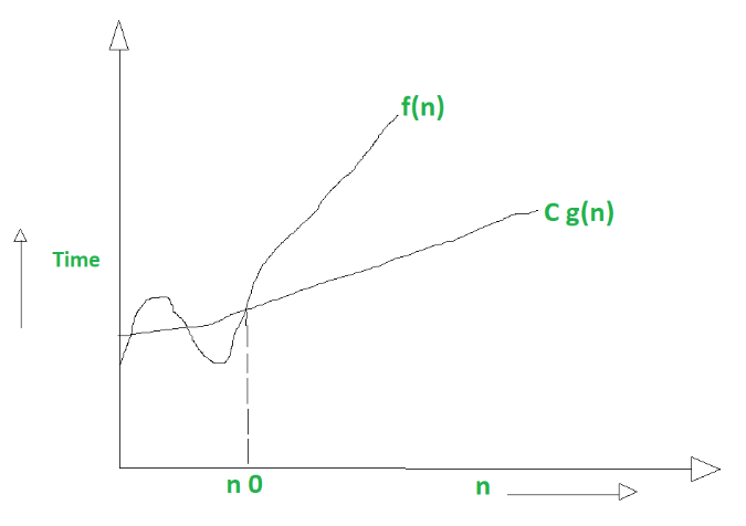
Big Omega ()
Describes the best-case scenario (lower bound):
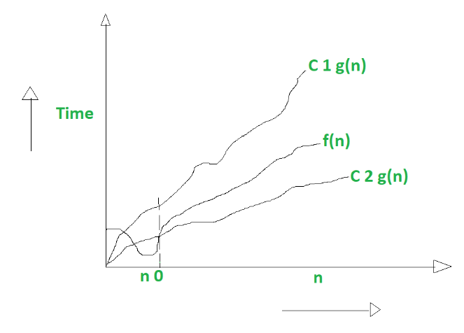
Big Theta ()
Describes the tightest bound (average case):
Summary
- Big is like (Worst case / Upper bound)
- Big is like (Best case / Lower bound)
- Big is like (Tightly bounded / Average case)
Determining what to optimize depends on your specific use case. A big factor to these algorithms is also input size, sometimes algorithms like bubble sort outperform ones like quicksort due to better cache locality (and aggressive compiler optimization because it’s a more predictable pattern) on small input sizes.